Help with Numbers formula

[Jmfocus]

Hello everone, I am new to the forum, recently purchased my first Ipad and here I am.

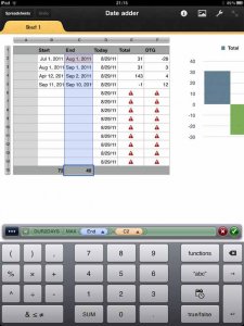
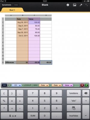
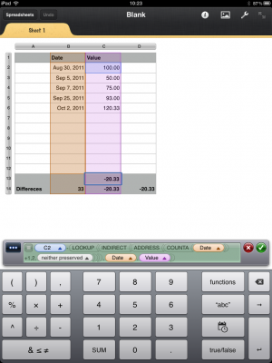
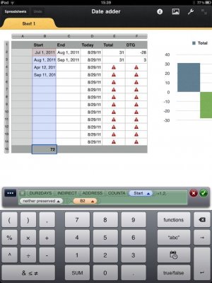
What I am trying to do is write a formula that will take the value of C2 and minus the most recent log entry at the bottom of column C and then updat in the footer. So that everytime I update the log, it updates the value in the footer. I have been researching this for days and can't get anything to work.

Thanks for your help

 

[twerppoet]

An interesting challenge. I'll give it a go. It would help if you could supply the basic file you want this to happen in (minus any private data) with a more detailed description of what exactly goes in what cell.

You'll need to make two more posts before you can post a link, so brows around in the forum and enjoy. You are bound to find something you want to comment on.

 

[Jmfocus]

Thanks Twerpoet. Basically I have a beginning number in C2 that corresponds with a date. Say that number is 100. Now in C3 there is a number 99. C4 has 98.65 etc. I have a footer that I would like to have update the differance between the first number "100" and the following numbers depending on the date of entry. So if 100 was input on 8/25 and 99 was input on 8/26 then the footer would read "1". On 8/27 the input number would be 98.65 and the footer would read 1.35 etc.

Hope that helps.

I think the formula would be C2- LOOKUP.... then something else that would grab the last entry in column C.

 

[twerppoet]

That sounds about right. I'll see what I can figure out.

 

[twerppoet]

Ok, here is what I came up with. It's not perfect, because it won't deal with gaps or cells with invisible entries (like spaces). You should be able to reduce the second by formatting the entire column as dates, and will just have to be careful about the first.


These instructions are inside out (first described, last done when creating the formula). Follow along best you can using the attached screen shot.

First you use COUNTA, to determine the number of entries in the column, add 1 to offset it to the actual row number (since it does not count the Header row. You select the row by taping the bar above the row, not one of the cells.

Next you use ADDRESS to turn the result into a location string. The COUNTA result becomes the row, and I manually enter a 2 for the column (because I'm using column B). Change the addr-type to 'neither preserved' to get a typical 'B5' result. Otherwise you end up with $B$5, which wont work with the next command. Carefully edit (delete) the other values and commas.

INDIRECT fetches the value of the cell address created by the ADDRESS function.

Subtract the beginning cell value from your your current value (or vise versa depending on whether you want negative or positive results. I opted for the former, because it was slightly easier to edit. (If you want the later, just insert the cursor before instead of after the formula, select the cell, and then tap minus). Hope that made sense. At any rate, the B2 would appear directly after DUR2DAYS instead of at the end of the equations, just before the last parentheses.

Finally the result needs to be a duration. I figured days (for a log) would be the most logical. DUR2DAYS converts the results of B5-B2 into the number of days.

Hope this helps.

 

[88raymond]

are the succeeding numbers always smaller than its predecessor? you can always use the minimum function

c2-min(c3:c99)

if not, if the dates are in column b,

=c2-vlookup(max(b2:b99),b2:c99,2)



note: this assumes your footer is on c100

 

[twerppoet]

are the succeeding numbers always smaller than its predecessor? you can always use the minimum function

c2-min(c3:c99)

if not, if the dates are in column b,

=c2-vlookup(max(b2:b99),b2:c99,2)



note: this assumes your footer is on c100

Thanks!

That's much better than my formula, as long as new entries are always either greater or lesser than the original date. I enclose it with the DUR2DAY function to get rid of the trailing d, and so the result will be a number that can be used in other equations.

I found it unnecessary to use VLOOKUP, since MAX returns the value directly. Or am I missing something?

My final formula, based on increasing dates from the original.

DUR2DAY(MAX(Dates)-C2) Where Dates is the name of the column. You can avoid using cell ranges if you select the entire column instead. Do this by tapping on the bar above the column instead of a cell. The function entry will become the Header of the column. As long as the formula is located in the footer, it will not be counted in the column range, and always at the bottom of the table.

EDIT: Added screen shot, just because I did it before. Note that in the screen shot the column's name is End, not Date. I thought I was being clever by changing the name to something that made more sense than my cobbled together test table.

 

[88raymond]

i don't have the ability to comprehend your solution, it seems too complex, hehe..

as i understand it, the OP has two sets of data: dates and values. each date has a corresponding value. he wants to always have the difference between the latest value entry with the original entry.

i assumed the latest entry would be the highest date value, thus the "max" function in my second formula. vlookup is needed because of the array (two sets of values).

 

[twerppoet]

Headsmack! You are right, the values, not the dates themselves are supposed to be compaired. I don't know where I got off track. I still think your formula will work better if you select the columns instead of a cell range, but have not tested it to be sure.

My first formula was way to complex, which is why I liked your use of MAX or MIN so much. I had not stumbled on those yet.

 

[twerppoet]

Ok, I had to go back and experiment some more. Maybe I've got some OCD hiding in my genes.

I could not get the column selection thing to work with your formula. However, when I used LOOKUP instead of VLOOKUP it worked just fine. Here is a screen shot of the results.

I do see one potential problem not mentioned yet. I don't know what the formula would do if you entered two identical dates. The results could be unpredictable. It could be avoided by entering the time as well, I suppose, but it would be easy to overlook.


Edit: Oops, notice I have D14 selected for the formula, but it is exactly the same formula instead as C14. I'd been playing with VLOOKUP in the D14 column because I was getting self-referencing errors in C14. I got it to work using LOOKUP, then copy pasted the formula to C14 where it worked just as well.

 

[twerppoet]

And finally, just because I am a total glutton for punishment, here is what it looks like if you go back to my method for finding the last entry in the table (as opposed to newest date).

Basically you replace the simple MAX statement with the INDIRECT statement (and everything inside it). Painful, unless you really need the last entry, and not just the most recent date.

 

[Jmfocus]

Guys thanks for helping me out. So far nothing is working. The solution below has been added to the footer line and shows only the actuall formula in the cell instead of making the computation.

The way my worksheet is set up is that everytime I add data it automatically adds a line to corrospond with the date. So I could have 500 entries when 500 days pass but the footer always remains at the bottom. I created the footer by touching the first cell in the spreadsheet which gives you the ability to maniputate the number of rows and columns, then touching the circle with a little "i" which brings up a window that will allow for a footer to be added and always kept at the bottom of the spreadsheet.

Twerppoet your solution was way over my head but thanks for your help. Do you guys think this is possible with the footer?

are the succeeding numbers always smaller than its predecessor? you can always use the minimum function

c2-min(c3:c99)

if not, if the dates are in column b,

=c2-vlookup(max(b2:b99),b2:c99,2)



note: this assumes your footer is on c100

 

[twerppoet]

Look at the second to last solution, not my very last. That was just an exercise in craziness. The only real difference between it and Raymond's solution is that I use the LOOKUP function instead of VLOOKUP, and I use column selections instead of cell ranges.

VLOOKUP kept including the header and footer cells in the search, so it failed when using columns. LOOKUP only sees the non-header/footer cells, so it could be set by tapping the entire column instead of needing to select a range of cells. This is more convenient since you don't have to worry about increasing the cell range latter if you make more entries than you originally planned.

C2-LOOKUP(Max(DateColumn),DateColumn,ValueColumn) Edit, fixed mistake. I got the two formulas mixed up. Sorry. It was correct in the screen shot though.

If that still does not make sense, here is the spreadsheet I've been playing with, with both the crazy and Raymond inspired simpler formulas. You can play with them until you understand what is going on.

 

[twerppoet]

BTW, what formula are you using to automatically set the date in a cell? I've been trying to figure out how to do this.

 

[Jmfocus]

Look at the second to last solution, not my very last. That was just an exercise in craziness. The only real difference between it and Raymond's solution is that I use the LOOKUP function instead of VLOOKUP, and I use column selections instead of cell ranges.

VLOOKUP kept including the header and footer cells in the search, so it failed when using columns. LOOKUP only sees the non-header/footer cells, so it could be set by tapping the entire column instead of needing to select a range of cells. This is more convenient since you don't have to worry about increasing the cell range latter if you make more entries than you originally planned.

C2-LOOKUP(Max(DateColumn),ValueColumn,2)

If that still does not make sense, here is the spreadsheet I've been playing with, with both the crazy and Raymond inspired simpler formulas. You can play with them until you understand what is going on.

Do I type that in as text exactly as you have it. If so, it doesn;t do the computation, it just shows the actual text in the footer cell.